

import json
import numpy as np
def simulate_regression(n=128, p=2, n_new=4, seed=145777):
def simulate_covariates(n):
x = rng.normal(size=(n, p))
x[:, 1] = x[:, 1]**2
return x
rng = np.random.default_rng(seed)
alpha = rng.normal(0.0, 5.0)
beta = rng.normal(0.0, 2.5, size=p)
sigma = rng.exponential(1.0 / 0.5) # numpy rng uses scale/mean parameterization
x = simulate_covariates(n)
mu = alpha + x @ beta
y = rng.normal(mu, sigma)
x_new = simulate_covariates(n_new)
parameters = { "alpha": alpha, "beta": beta, "sigma": sigma }
data = {
"N": n, "P": p, "N_new": n_new, "x": x.tolist(),
"y": y.tolist(), "x_new": x_new.tolist(),
}
return parameters, data
params, data = simulate_regression()1 Motivation
1.1 Bayesian workflow
Gelman et al. (2013) begin their foundational textbook by factoring Bayesian data analysis into three steps.
- Design a joint probability distribution for observable data and unobservable parameters.
- Perform inference to generate a posterior sample over parameters and unobserved data conditioned on observed data.
- Evaluate the model fit and what it tells us about our quantities of interest.
The authors further suggest that if the evaluation in step (3) is not sufficient, then one should go back to step (1) and try to come up with a better model. More recently, Gelman et al. (2020) outlined a workflow for Bayesian analysis that puts more emphasis on fitting multiple models and transparently reporting their exploration and comparison.
A probabilistic programming language (PPL) primarily provides support for statisticians who wish to code a statistical model defined in step (1) so that it can be used for inference in step (2). The PPL syntax allows for a straightforward encoding of the joint probability distribution. PPLs are typically coupled with samplers that allow step (2) to be performed with Monte Carlo methods and are coupled with posterior analysis and model comparison tools for task (3). In addition, once the log unnormalized density is set up, PPLs can compute other operations such as mode finding, Laplace approximation, and variational inference.
In this paper, we are going to focus on specifying models and performing posterior sampling as is done by a PPL, but without actually using a PPL. We will also provide guidance on integration with tools for inference, model evaluation/criticism, and model comparison. Our goal is to develop a methodology for implementing efficient and scalable differentiable Bayesian models in Python in a way that is both easy to code and easy to read.
For step (2), we recommend the Python package Blackjax (Cabezas et al. 2024). Blackjax includes implementations of Stan’s primary inference methods, the no-U-turn sampler (NUTS) (Hoffman and Gelman 2014), automatic differentiation variational inference (ADVI) (Kucukelbir et al. 2017), and Pathfinder variational inference (Zhang et al. 2022). Blackjax is being actively maintained and extended, and already includes several other useful algorithms, including microcanonical (aka isokinetic) sampling (Robnik et al. 2025), sequential Monte Carlo (SMC) (Doucet et al. 2001), elliptical slice sampling (Murray et al. 2010), generalized HMC (GHMC) (Horowitz 1991), and even random-walk Metropolis (RWM) (Hastings 1970).
For step (3), we recommend the Python package Arviz (Kumar et al. 2019). Arviz provides state-of-the-art convergence monitoring using split, ranked \widehat{R}, estimation of bulk and tail effective sample sizes, standard errors, posterior means, standard deviations, and quantiles, as well as approximate leave-one-out (LOO) cross-validation (Vehtari et al. 2021, 2017).
1.2 Why not just use Stan?
Stan (Carpenter et al. 2017) is a domain-specific language for expressing differentiable probability densities and posterior predictive quantities. Stan is a probabilistic programming language in the sense that its variables can be interpreted as random variables. Stan has been used in almost every area where statistics is applied, and as such, has accumulated an unmatched depth and breadth of training materials around different classes of probabilistic models. There are textbooks, college classes, and reproducible case studies in all of these areas. There’s a vibrant community with a high volume discussion forum. The language is still being expanded and so is it’s math library.
The Stan project introduced several state of the art gradient-based inference algorithms including the no-U-turn sampler (NUTS) (Hoffman and Gelman 2014), automatic differentiation variational inference (ADVI) (Kucukelbir et al. 2017), Pathfinder variational inference (Zhang et al. 2022), and black-box nested Laplace approximations (Margossian 2023) as well as posterior analysis tools such as split- and ranked-\widehat{R} and corresponding bulk and tail effective sample size (Vehtari et al. 2021), leave-one-out cross-validation (Vehtari et al. 2017), refined simulation-based calibration checks (Cook et al. 2006), and prior predictive checks (Gabry et al. 2019). It is often used as the basis of methodological developments such as Bayesian workflow (Gelman et al. 2020).
So why not just use Stan? The first reason is that Stan is largely CPU-bound. All of its analysis tools and algorithms run on the CPU. Although there are ways to call individual functions in a Stan program on the GPU (e.g., Cholesky decomposition) and ways to apply map-reduce across multiple cores, this is not enough. Stan lacks a way to keep computation in-kernel on the GPU or organize inference to enable single-instruction multiple-data (SIMD) parallelism. Although Stan has been faster than JAX on CPU, it is not competitive on modern hardware (Sountsov et al. 2024; Maskell 2024).
The second obstacle to using Stan is the need to learn a second language. While Stan is not particularly complicated, it does present several additional difficulties beyond unfamiliar syntax and semantics.
- Stan is indexed from 1, like much of mathematics and in particular, linear algebra, whereas Python is indexed from 0, like most programming languages. Translating between 0-based and 1-based indexing is tedious, error-prone, and obfuscates code.
- Stan is strongly typed and statically compiled, which has the benefit of being type-safe at run time and leads to fast C++ computation. The downside is that this kind of static typing is unfamiliar to most of Stan’s intended users. Stan’s typing can be an annoyance and performance bottleneck even for experienced programmers due to its poor representational choice for containers that mixes C++ standard vectors (Josuttis 2012) for arrays and Eigen matrices (Guennebaud and Jacob 2010) for linear algebra (this may sound harsh, but it was our fault as the original developers of Stan).
- Stan requires a scripting language like R, Python, and Julia, to combine modeling with data preparation and posterior analysis, rather than providing a seamless single-language experience. The interface between these languages and Stan is minimal—Stan is just being called as a black box to return samples.
- There is relatively little tooling to aid with Stan development. Currently, it’s just autocomplete, syntax highlighting, and debug-by-print. Python, in contrast, has several well supported integrated development environments with tooling for debugging, generating notebooks, integration with chatbots, integration with documentation, automatic refactoring tools, etc.
- While there is a great deal of tutorial and onboarding material for Stan, it has to split its attention among several interfaces (two interfaces in R and Python and one in Julia). Taken together, even Stan’s extensive documentation is dwarfed by the pedagogical material around scientific, differentiable, and probabilistic computing in Python.
1.3 Why not just use PyMC or NumPyro?
The very first probabilistic programming language of which we are aware is BUGS (Bayesian inference using Gibbs Sampling) (Lunn et al. 2009, 2012), which was released way back in 1991. In BUGS, Bayesian models are specified with deterministic and stochastic nodes arranged in a directed acyclic graph. Each node was either input as data, or defined as a (possibly stochastic) function of its direct ancestors in the graph. This enabled a BUGS model to be used to infer any of the stochastic variables in the model given values for the data nodes and all other stochastic nodes. This provides a clean way to perform analyses such as prior predictive inference and posterior predictive inference automatically through the graphical structure of the model. BUGS samples using generalized Gibbs sampling, which does not scale well in dimension.
PyMC (Salvatier et al. 2016) and NumPyro (Phan et al. 2019) are Python packages that take a directed graphical modeling approach to specifying Bayesian models and are capable of generating JAX code as output. There are similar packages in other languages, but they do not generate JAX code. JAGS (Plummer 2003) is a standalone language that reimplements and extends BUGS and is typically used through R, NIMBLE (Valpine et al. 2017) is coded in R, and Turing.jl (Ge et al. 2018) is coded in Julia.
Like Stan, all of the modern PPLs efficiently scale in dimension by using gradient-based inference methods. Like BUGS, they are able to exploit the graphical model structure directly to automate a number of functions that are painful to code in Stan and will largely remain painful to code in what we are proposing here, such as prior and posterior predictive checks and simulation-based calibration, and at least in the case of PyMC, general patterns of missing data.
When models get more complicated in terms of novel parameter constraints, densities, conditional structures, etc., both PyMC and NumPyro provide escape hatches to let you define transformations and log densities directly in the same way as Stan. This feels dirty in the same way as using the “ones-trick” in BUGS (Lunn et al. 2012). And while it is great for allowing general models to be defined, it defeats all the benefits of having a clean generative graphical model in the first place. At the point models start getting more complicated, we believe it is more straightforward to code the models directly in JAX rather than working around the graphical modeling paradigm of PyMC or NumPyro.
A second reason to prefer the approach we are presenting here is that it is much more direct. By that, we mean that like Stan, the resulting code is implemented transparently in an imperative fashion rather than indirectly through the structure of the directed acyclic graph.
1.4 Special function support in JAX
Stan has an extensive library of special mathematical and statistical functions, as well as restructuring functions for arrays and matrices. Many of these are needed to differentiate cumulative distribution functions and to define custom densities. Here’s a brief overview of the coverage available in JAX compared to Stan. The bottom line is that support for special functions is deeper in JAX.
Matrix library: This is JAX’s main focus and it far exceeds Stan’s collection of familiar matrix functions and reshaping tools by punning NumPy (
jax.numpy) and SciPy (jax.scipy). There is even limited (and experimental) support for sparse matrices and solvers natively (jax.experimental.sparse).Special functions: These are available all over the JAX ecosystem, including in JAX’s NumPy and SciPy modules. The differentiable SciPy module (
jax.scipy.special) is not complete compared to SciPy. The deficit is more than made up by the special function library provided by TensorFlow Probability (TFP) (tfp.math) and maintained by Google. For example, the Lambert W function available in Stan has not been ported from SciPy but is available through TFP. The bottom line is that JAX provides a better selection of well supported special functions.Probability distributions: Stan implements dozens of probability distributions, including most (but not all) of the ones in common use for statistical models. While the basics are available through JAX’s NumPy and SciPy modules (often redundantly), the go-to library is TensorFlow Probability (TFP) (e.g.,
tfp.distributions; for JAX specifically,tfp.substrates.jax.distributions) for probability-related functions (e.g., probability density functions, probability mass functions, and cumulative distribution functions). In some cases, there are also quantile functions, which are poorly supported in Stan. The bottom line is that the native Google-supported JAX ecosystem provides a better selection of well supported probability functions and random number generators. There is even wider support beyond native JAX and TensorFlow, including the probabilistic programming language NumPyro (Phan et al. 2019) and Google DeepMind’s library Distrax (DeepMind et al. 2020).Complex-valued functions: JAX and Stan both have core library support for complex-valued functions built-in, including fast Fourier transforms and complex matrix operations.
Neural networks: JAX is integrated tightly with a range of neural network constructions through the Flax package (Heek et al. 2024), which is maintained by a team at Google DeepMind, but is not an official Google product like TensorFlow or JAX. It supports everything from simple multilayer perceptrons and convolutional neural networks to autoencoders and multi-head attention.
Simulation-based inference (SBI): There is as of yet, no mature and commonly used SBI package in JAX, nor is there any support in Stan.
Implicit Solvers: Applied statistics often requires equations to be solved and differentiated and Stan provides a fairly extensive library.
Ordinary differential equation (ODE) solvers: There is no built-in support in JAX for ODE solvers, but the Diffrax package (Kidger 2021) is widely used and provides the same kind of adjoint and analytic methods as Stan that provide sensitivity analysis without automatically differentiating through the algorithm.
Root finders: There is no built-in support in JAX for root finders, but the JAXOpt package (Blondel et al. 2021) is maintained by Google and provides a range of solvers including the Newton method used by Stan.
1D Integration: These functions are useful for defining cumulative distribution functions for novel densities. JAX does not ship an adaptive 1D quadrature routine in core, but external libraries such as
quadaxprovidejit/vmap-able, differentiable adaptive quadrature (e.g., Gauss–Kronrod-stylequadgk).Hidden Markov models: TFP (through
tfp.distributions.HiddenMarkovModel) supports likelihood evaluation (forward algorithm) and computation of latent-state marginals (a form of the forward–backward algorithm, e.g.posterior_marginals). Stan provides analogous built-ins (hmm_marginalfor the marginal likelihood andhmm_hidden_state_probfor marginal latent state probabilities).Kalman filters: Stan has direct support for Gaussian dynamic linear model likelihoods computed via the Kalman filter (e.g.,
gaussian_dlm_obs_lpdfand related functions). There is also experimental support in TFP (intfp.experimental.parallel_filter.kalman_filter).Partial differential equation (PDE) solvers: Stan has no support for partial differential equations. The JAX-CFD package (Kochkov et al. 2021) from Google, mostly focused on fluid dynamics, includes a number of general-purpose PDE solvers, including finite volume/difference methods, pseudospectral methods, and machine-learning methods. It supports Navier-Stokes, advection-diffusion, period and wall boundary conditions, and runs on GPU and TPU with gradients.
Stochastic differential equation (SDE) solvers: Stan has no support for stochastic differential equations. The Diffrax package (Kidger 2021), in addition to providing stiff ODE solvers, also supports traditional SDE and SPDE solvers (Eueler-Maruyama, Milstein, Stratonovich/Itô) through spatial discretization.
With the caveat that functionality is spread across multiple libraries (core JAX, TFP, and smaller add-ons such as quadax for adaptive quadrature), the special function, probability distribution, and transform coverage available in the JAX ecosystem is broadly comparable to Stan’s, and in some areas deeper. When it comes to even more complicated functions like PDE and SDE solvers and neural networks, Stan isn’t even in the game. The JAX-based PPL NumPyro can also make use of these JAX packages in many cases, especially if users are willing to forego its underlying graphical model abstraction.
1.5 Constrained parameter support in JAX
Stan provides built-in transforms that map an unconstrained vector in \mathbb{R}^d into a desired constrained space (e.g., a (d+1)-simplex), along with the corresponding change-of-variables adjustments to the density. These are custom implementations with analytic Jacobian-adjoint product gradients and vectorized application to containers.
The Oryx transform library in TensorFlow is built on top of the TFP bijector library (tfp.bijectors) (Dillon et al. 2017), which can also be used directly. TFP bijectors provide all of the transforms provided by Stan and many more including softplus, various cdfs and hyperbolic tangent as replacements for inverse-logit, more multivariate transforms such as cumulative sums and Householder factorizations, as well as trained transforms like RealNVP normalizing flows (Dinh et al. 2016). Oryx additionally allows transforms to be written down directly in such a way that Oryx can automatically calculate inverse transforms and Jacobian determinants of inverse transforms.
1.6 Modularity in JAX
SlicStan (Gorinova et al. 2019) reconceived Stan without blocks—the sorting into data, parameters, and generated quantities was carried out by data flow analysis. The primary motivation was to make it possible to modularly express concepts like a hierarchical prior. With Stan itself, this is impossible unless the modularity is in the form of a simple function. With SlicStan, the parameters, priors, etc., could all be constructed modularly and reused. By allowing models to be expressed directly in Python code, NumPyro and PyMC already support modular code reuse. Although it is rare to see this feature used in example code, it is widely used in production.
By coding models directly in Python, we gain the same benefits of NumPyro and PyMC. We can write general programs returning arbitrary components of a probabilistic program and combine them at will. We will provide examples below.
2 Bayesian inference
In this section, we will lay out the precise definition of the Bayesian inference problem we are trying to compute, show how it can be computed asymptotically exactly using Monte Carlo methods, and apply some simple calculus to transform parameterizations to be unconstrained (i.e., have support over all of \mathbb{R}^D).
2.1 Bayesian models
A Bayesian model is a joint distribution over parameters \theta and data y.
In the simplest version of this formulation, Bayesian inference uses the posterior distribution of the parameters given the data: p(\theta \mid y) \propto p(\theta, y). Often our density is factored into a prior times a likelihood, p(\theta \mid y) = p(\theta) \cdot p(y \mid \theta), but nothing in Stan or what we are proposing for JAX presupposes a clean factorization. In fact, our methods can be used to sample from any unnormalized density with finite integral—it doesn’t have to arise as a Bayesian posterior.
More generally, if “data” are defined as observable quantities, there can be observed data y^{\rm obs} and unobserved data y^{\rm mis} (short for “missing data” but this can also include latent (unobserved but potentially observable) data, future data, unrecorded past data, etc.), and Bayesian inference uses the posterior distribution of all unobserved quantities conditional on observed data, thus p(\theta, y^{\rm mis} \mid y^{\rm obs}). There is no strict rule for what aspects of a model count as “parameters” and what count as “data.” But Bayesian inference doesn’t really care if an unknown quantity is put in the “\theta” bin or the “y^{\rm mis}” bin; all that matters is what is being conditioned on.
In that case, why not just label everything unknown in a problem as “parameters” and everything observed as “data”? You can do this; indeed, that’s how variables are coded in Stan. The trouble with using this as a general dividing line is that, the knowledge of what is observed and what is not observed can be logically independent of the model. For a simple example, start with data y_1,\dots,y_N from a first-order autoregressive model with parameters a,b,\sigma. Now suppose that you want to make predictions for future data, y_{N+1},\dots,y_{N+10}. It would be awkward to label these new data points as parameters, even though they are unknown.
2.2 Generative modeling
In Bayesian terminology, the joint distribution, p(\theta,y) = p(\theta)p(y \mid \theta), is a generative model, because a random \theta can be generated from the prior and a random y can be generated from the data distribution. For complicated models the generation process can be further divided; for example, in a hierarchical model with local parameters \alpha and hyperparameters \phi, so that \theta=(\phi, \alpha), the joint distribution can be factored as p(\phi)p(\alpha \mid \phi)p(\theta \mid \phi,\alpha) which corresponds to the generated process in which \phi, \alpha, and y are simulated in order. As models become even more complicated, it can be helpful to express the factorization as a directed acyclic graph, and the joint distribution is called a graphical model.
2.3 Unmodeled data
So far we have discussed parameters \theta, observed data y^{\rm obs}, and latent or unobserve data y^{\rm mis}. Bayesian models typically also include unmodeled data, for example the sample size and predictors in a regression model. If we write all the unmodeled data as x, then the posterior is p(\theta, y^{\rm mis} \mid y^{\rm obs}, x). This is not a full generative model because there is no distribution for x.
Different probabilistic programming languages handle unmodeled data in different ways.
A Stan program computes the target function—the unnormalized log posterior density function, and there is no logical distinction between y^{\rm obs} and x: both are input to the program as data. Indeed, there is no logical distinction between \theta and y^{\rm mis}, although for computational efficiency it is best to simulate y^{\rm mis} in the generated quantities block if possible.
In contrast, a PyMC program specifies a graphical model for (\theta,y \mid x), and it can be run to simulate any subset of (\theta,y), conditional on x and whatever information is passed in as data: for example, specify nothing but x and it will simulate from the joint distribution; specify \theta and x and it will simulate y from the data model; specify y and x and it will simulate \theta from the posterior.
In any probabilistic programming language, you need to specify the unmodeled data. But it is also possible, and often recommended, to expand to include a model for x.
2.4 Bayesian inference with posterior expectations and simulations
Bayesian inference involves visualizing and summarizing quantities of interest in the posterior and posterior predictive distributions. For summaries, we are typically interested in posterior averages or posterior quantiles of parameters, predictions, or some functions of parameters and data. Quantiles are typically used to give us medians and uncertainty intervals, while averages give us everything else. By averaging estimates of quantities of interest derived from parameters weighted by posterior density, we can account for estimation uncertainty into account in our inferences.
Averages over the posterior density are most naturally expressed using expectation notation. Given a random variable \Theta \in \mathbb{R}^D representing knowledge about the parameters, the expectation of a function f:\mathbb{R}^D \rightarrow \mathbb{R} is given by \mathbb{E}[f(\Theta) \mid y] = \int_{\mathbb{R}^D} f(\theta) \cdot p(\theta \mid y) \, \textrm{d}\theta. The rest of this section provides examples of common functions whose expectations are evaluated for Bayesian inference.
The parameter estimate that minimizes expected square error, assuming the model is correct, is the posterior mean, \widehat{\theta} = \mathbb{E}[\Theta \mid y]. This is just taking the function f to be the identity. The posterior covariance is \textrm{var}[\Theta \mid y] = \mathbb{E}[(\Theta - \widehat{\theta}) \cdot (\theta - \widehat{\theta})^\top]. Here the function is f(\theta) = (\theta - \widehat{\theta}) \cdot (\theta - \widehat{\theta})^\top..
If we have an event A \subseteq \mathbb{R}^D, then its probability is given by the expectation of its indicator function, \Pr[\theta \in A \mid y] = \mathbb{E}[\mathbb{1}_A(\theta \in A) \mid y].
If we want to evaluate posterior predictive densities p(\tilde{y} \mid y) for new data \tilde{y}, this can be expressed as an expectation of the likelihood p(\tilde{y} \mid \theta), p(\tilde{y} \mid y) = \mathbb{E}[p(\tilde{y} \mid \theta) \mid y].
We can reduce the high-dimensional integration problem to one of sampling from the posterior, \theta^{(m)} \sim p(\theta \mid y). Given independent and identically distributed (i.i.d.) Monte Carlo draws, the Monte Carlo estimator \widehat{I}_M \;\;=\;\; \frac{1}{M}\sum_{m=1}^{M} f(\theta^{(m)}) converges almost surely (with probability 1) to the true posterior expectation \mathbb{E}[f(\Theta)\mid y] by the strong law of large numbers. Moreover, if \textrm{var}[f(\Theta)\mid y] < \infty, then a central limit theorem gives the asymptotic normal approximation \sqrt{M}\Big(\widehat{I}_M - \mathbb{E}[f(\Theta)\mid y]\Big) \quad\text{converges in distribution to}\quad \mathcal{N}\!\left(0,\;\textrm{var}[f(\Theta)\mid y]\right), which implies the familiar \mathcal{O}(1/\sqrt{M}) Monte Carlo error rate. Finite-sample concentration bounds also hold under additional regularity assumptions (e.g., boundedness or sub-exponential tails of f(\Theta)), giving us explicit deviation probabilities for \widehat{I}_M around \mathbb{E}[f(\Theta)\mid y] (Gelman et al. 2013; Paulin 2015).
In practice, we often summarize Bayesian inference using posterior simulations, without deciding ahead of time what expectations or other posterior summaries will be needed. So it is convenient that, with a large number of independent draws from the posterior distribution of all parameters and unobserved data of potential interest, we can use these to estimate arbitrary expectations, as well as obtain an estimate of their Monte Carlo uncertainty.
In addition, posterior simulations can be used for multiple imputation of missing data (Rubin 1996) and to understand the fitted model. For example, in a logistic regression model, Pr(y=1|x)=\textrm{logit}^{-1}(a + bx), one can make a scatterplot of posterior simulations of (a,b), along with a graph of data (x,y)_n, n=1,\dots,N along with curves, \textrm{logit}^{-1}(a + bx) corresponding to those draws of (a,b).
2.5 Computation with Markov chain Monte Carlo methods
In practice, exact independent draws from p(\theta\mid y) are rarely available. Fortunately, many weaker sampling schemes still yield consistent estimators of posterior expectations. These include rejection sampling and importance sampling (which produce weighted estimators), sequential Monte Carlo (which propagates and reweights a particle population), and Markov chain Monte Carlo (which constructs a dependent sequence whose stationary distribution is the posterior) (Gelman et al. 2013; Doucet et al. 2001; Roberts and Rosenthal 2004).
The idea of Markov chain Monte Carlo (MCMC) is that correlated draws from an ergodic Markov chain whose invariant (stationary) distribution is p(\theta\mid y) can still be used in the same sample-average estimator \widehat{I}_M. Under standard conditions (e.g., Harris ergodicity) that are easily satisfied in practical applications, the Markov chain ergodic theorem guarantees \widehat{I}_M \to \mathbb{E}[f(\Theta)\mid y] even though the draws are dependent (Roberts and Rosenthal 2004).
When the chain is particularly well behaved (e.g., geometrically ergodic with suitable moment conditions) a Markov chain central limit theorem holds: \sqrt{M}\Big(\widehat{I}_M - \mathbb{E}[f(\Theta)\mid y]\Big) \quad\text{converges in distribution to}\quad \mathcal{N}\!\left(0,\;\sigma_f^2\right), with asymptotic variance \sigma_f^2 = \textrm{var}_\pi(f(\Theta))\ \tau_\text{int}, where \pi(\cdot)=p(\cdot\mid y), \{\Theta_k\} denotes the stationary chain, and \tau_\text{int} (the integrated autocorrelation time) satisfies \tau_\text{int}=1+2\sum_{k\ge 1}\textrm{corr}_\pi\!\big(f(\Theta_0), f(\Theta_k)\big). This motivates defining the effective sample size as M_\text{eff}=M/\tau_\text{int} and using the heuristic \mathcal{O}(1/\sqrt{M_\text{eff}}) error rate (Roberts and Rosenthal 2004; Vehtari et al. 2021). Under similarly strong assumptions (e.g., uniform or geometric ergodicity, or a spectral-gap condition), one can also obtain non-asymptotic deviation bounds and Bernstein- or Hoeffding-type concentration inequalities for Markov chain averages (Paulin 2015).
These strong conditions needed for MCMC central limit theorems and concentration bounds are typically difficult to verify for the complex MCMC methods and posteriors encountered in modern Bayesian inference over continuous parameter spaces (Roberts and Rosenthal 2004). Even so, MCMC, especially modern gradient-based variants, has shown remarkable empirical success in applied Bayesian inference. Instead of verifying theoretical assumptions, users tend to assess practical reliability via convergence diagnostics, effective sample sizes, and predictive checks (Gelman et al. 2020; Vehtari et al. 2021).
2.6 Unconstrained parameterizations
It is much easier to define a sampling algorithm (particularly a gradient-based sampler like HMC/NUTS) when the sampler’s state lives in an unconstrained Euclidean space \mathbb{R}^N, with no hard boundaries. Stan and other PPLs achieve this by representing each constrained parameter \Theta\in C\subseteq\mathbb{R}^D using an unconstrained variable \Phi\in\mathbb{R}^N and a smooth map t:\mathbb{R}^N \to C,\qquad \Theta = t(\Phi), so we can run the sampler in \phi-space and interpret \theta=t(\phi) on the constrained space C. Here N is the number of unconstrained degrees of freedom chosen for the parameterization; for example, for a K-simplex one typically chooses N=K-1 with a stick-breaking parameterization t. This requires an adjustment for the change of variables, which happens implicitly in PPLs. Stan requires all parameter constraints to be declared; the graphical modeling sublanguage of PyMC and NumPyro infer these constraints from the distributions in which variables participate (e.g., if a variable is given a Wishart distribution, it must be a symmetric and positive definite matrix).
2.6.1 The common case of constraints via bijections
Mathematically, in the common one-to-one case where t is a smooth bijection onto C (so it has a smooth inverse f=t^{-1}:C\to\mathbb{R}^N), given a constrained random variable \Theta \in C with a density p_\Theta(\theta), we can derive the density of \Phi = f(\Theta) as p_\Phi(\phi) = p_\Theta(f^{-1}(\phi)) \cdot \left|\det D f^{-1}(\phi)\right| = p_\Theta(t(\phi)) \cdot \left|\det Dt(\phi)\right|, where Df^{-1}(\phi) (equivalently Dt(\phi)) denotes the Jacobian matrix at \phi, and |\det(\cdot)| denotes the absolute value of the determinant. In the univariate case, \det Df^{-1}(\phi) reduces to (f^{-1})'(\phi).
If there is a sequence of variables being transformed one at a time, the overall Jacobian will be block diagonal, with an absolute Jacobian determinant equal to the product of the absolute Jacobian determinants of the blocks. Unconstrained parameters are transformed by the identity, which has a unit Jacobian determinant. This makes it particularly simple to work on the unconstrained scale—we just map unconstrained parameters back to the constrained space using the inverse (constraining) transforms and add the log absolute determinants of their Jacobians. For maximum likelihood estimation, the Jacobians can be dropped from the target density with a flag.
2.6.2 Transforms as parameterizations (not just “constraints” or “bijectors”)
It can be helpful to think of Stan’s constraints and TensorFlow Probability’s bijectors as instances of a broader modeling choice: a parameterization t:\mathbb{R}^N\to C. From this viewpoint, the names are a bit misleading: t need not encode a “constraint” (for example, affine maps t(z)=\mu+Lz map \mathbb{R}^D to all of \mathbb{R}^D and are central to non-centered parameterizations), and t need not be one-to-one (for example, the map t(z)=z/\|z\| can give a useful parameterization of distributions on spheres). Even for a fixed space C, there can be multiple useful parameterizations with different numerical behavior (for example, \exp versus \mathrm{softplus} for (0,\infty), logit versus probit links for (0,1), and stick-breaking versus softmax-style constructions for a simplex).
From an implementation point of view it is often convenient, most importantly for initializing parameters, to also provide a transform f:C\to\mathbb{R}^N that goes in the opposite direction. When t is not one-to-one this cannot be a true inverse; instead we often want it to behave as a (right inverse) in the sense that t\bigl(f(\theta)\bigr)=\theta,\qquad \theta\in C, i.e. t\circ f=\mathrm{id}_C. This is particularly useful for initialization: if we want to initialize the constrained parameter to \theta_0\in C, we can initialize the unconstrained parameter to \phi_0=f(\theta_0), which yields the desired initialization on the constrained side, t(\phi_0)=t(f(\theta_0))=\theta_0.
As long as C\subseteq \mathbb{R}^D is an embedded submanifold of dimension d, it admits a canonical notion of d-dimensional volume, generalizing the usual notion of volume d\theta on \mathbb{R}^D. We can think of this volume d\theta as a (possibly improper) unnormalized uniform prior on C. We can consider probability distributions on C arising from density functions w.r.t. this notion of volume. For example, if C is compact (i.e., if it is contained in a ball of some finite radius), we have a canonical notion of uniform distribution. A user of a PPL would expect the default density w.r.t. d\theta on the type C to be 1 (so log-density 0) when nothing is specified. Further, for intuitive use, any (log-)densities specified by the user on \theta of type C should also be relative to d\theta.
Therefore, our goal as PPL designers is to find a density g^t with respect to the volume d\phi on \mathbb{R}^N that induces our canonical volume d\theta on C via t in the sense that, for any integrable function h:C\to \mathbb{R}, \int_{\phi\in \mathbb{R}^N} g^t(\phi) h(t(\phi)) d\phi = \int_{\theta\in C} h(\theta) d\theta. (In technical terms: g^t\cdot d\phi pushes forward to d\theta along t.)
2.6.3 Density corrections beyond one-to-one maps
The Jacobian-determinant correction above is the special case where t is one-to-one. If t is many-to-one, the correction must also account for redundancy: how many unconstrained points represent the same constrained value.
Assume that C\subseteq \mathbb{R}^D is an embedded submanifold of dimension d. Further assume that t is smooth and regular in the sense that, at points we care about, small changes in \phi can move \theta=t(\phi) in all d local directions available inside C. Put differently, let Dt(\phi) denote the Jacobian matrix of t in the coordinates given by the inclusion C\subseteq \mathbb{R}^D, and assume that the induced linear map D^C t(\phi):\mathbb{R}^N\to T_{t(\phi)}C is surjective. Let s_1(\phi),\dots,s_d(\phi) be the positive singular values of Dt(\phi). Then, define the coarea “Jacobian factor” J_t(\phi) \;=\; \prod_{i=1}^{d} s_i(\phi)\; = \; \sqrt{\det(D^C t(\phi)D^C t(\phi)^\top)}, which reduces to \left|\det Dt(\phi)\right| when N=d and t is locally one-to-one. Also define the set of representations (preimages) of a point \theta\in C, t^{-1}(\theta)=\{\phi\in\mathbb{R}^N: t(\phi)=\theta\}, and the natural volume element d\phi_\perp along the preimage such that d\theta and d\phi_\perp give the orthogonal decomposition of d\phi along C and perpendicular to C within \mathbb{R}^N. The coarea formula of multivariate calculus then tells us that for any integrable function k:\mathbb{R}^N\to \mathbb{R}, \int_{\phi\in \mathbb{R}^N} k(\phi) J_t(\phi) d\phi = \int_{\theta\in C} \left(\int_{\phi\in t^{-1}(\theta)} k(\phi) d\phi_\perp\right) d\theta. In particular, if h:C\to \mathbb{R} is integrable and g^t_\perp is some function that restricts to a probability density on t^{-1}(\theta) for each \theta\in C, then \int_{\phi\in \mathbb{R}^N} h(t(\phi)) g^t_\perp(\phi) J_t(\phi) d\phi = \int_{\theta\in C} h(\theta) \left(\int_{\phi\in t^{-1}(\theta)} g^t_\perp(\phi)d\phi_\perp\right) d\theta = \int_{\theta\in C} h(\theta) d\theta, as desired. That is, to induce our desired default volume on C, we can use on \mathbb{R}^N the canonical density g^t(\phi)\;=\; J_t(\phi) g^t_\perp(\phi). Consequently, if a model specifies an (unnormalized) density \tilde{p}(\theta) on C relative to the canonical volume on C, then an equivalent (unnormalized) log-density target on \mathbb{R}^N is \log \tilde{p}(t(\phi))\;+\;\log J_t(\phi)\;+\;\log g^t_\perp(\phi).
In particular, if all t^{-1}(\theta) are compact, we can take $ gt_()=V(t()){-1} $ where the volume V(\theta) is defined as V(\theta) = \int_{t^{-1}(\theta)} d\phi_\perp. In general, however, there is freedom in the choice of g^t_\perp.
Two special cases are worth keeping in mind:
One-to-one: V(\theta)=1, so we recover the usual \log|\det Dt(\phi)| correction.
k-to-one with (almost everywhere) constant k: V(\theta)=k almost everywhere, so we can take g^t_\perp inversely proportional to the volume and the extra term is just -\log k, a constant that does not affect MCMC. Example: t(\phi)=\phi^2 maps \mathbb{R}\to(0,\infty) and is two-to-one away from 0.
Overparameterized maps can also have preimages of non-compact positive dimension (e.g., softmax logits without a centering convention, or the z\mapsto z/\|z\| parameterization of unit vectors). In such cases one is forced to make some choice of a density g^t_\perp so that the induced target on \mathbb{R}^N is well defined.
Stan supplies constraints for variables that are lower bounded (for scales), upper bounded (for log probabilities), range bounded (for probabilities), affine transforms (for non-centered parameterizations), ordered vectors (for cutpoints in ordinal regressions or identifying mixtures), unit vectors (for points on a hypersphere), simplices (for categorical probability distributions), sum-to-zero vectors (for identifying varying effects), positive-definite symmetric matrices and their Cholesky factors (for covariance or precision matrices), and for unit-diagonal positive-definite matrices and their Cholesky factors (for correlation matrices). The Oryx package, which is native to JAX and built on top of the TensorFlow Probability bijectors package (Dillon et al. 2017), provides an even wider range of useful transforms than Stan (e.g., softplus, alternative sigmoid cdfs, tanh, autoregressions, and flows, and many many more).
3 Coding models in Stan
To ground the discussion, let’s consider the concrete example of coding a linear regression and using it to predict new observations.
3.1 A multivariate linear regression model
We will assume a very simple multivariate regression formulation with an intercept, P \in \mathbb{N} covariates, and N \in \mathbb{N} observations. Our data is made up of observations y_n \in \mathbb{R} paired with covariates x_n \in \mathbb{R}^{N \times P}. We will assume the usual parameters consisting of a slope \alpha \in \mathbb{R}, regression coefficients \beta \in \mathbb{R}^P, and an error scale \sigma \in (0, \infty). We will assume the data and covariates are approximately on unit scale so that we can consider the following prior as weakly informative: \alpha \sim \textrm{normal}(0, 5) \qquad \beta_p \sim \textrm{normal}(0, 2.5) \qquad \sigma \sim \textrm{exponential}(0.5). We then add the conventional data generating process with independent normal errors, y_n \sim \textrm{normal}(\alpha + x_n \cdot \beta, \sigma). The joint density defining our Bayesian model (with data x taken as an unmodeled constant) is thus \textstyle \begin{array}{rcl} p(y, \alpha, \beta, \sigma \mid x) & = & \textrm{exponential}(\sigma \mid 0.5) \cdot \textrm{normal}(\alpha \mid 0, 5) \\[4pt] & & {} \cdot \left( \prod_{p=1}^P \textrm{normal}(\beta_p \mid 0, 2.5) \right) \cdot \left( \prod_{n=1}^N \textrm{normal}(y_n \mid \alpha + x_n \cdot \beta, \sigma) \right). \end{array} Bayes’s rule allows us to use the joint density as an unnormalized posterior, p(\alpha, \beta, \sigma \mid y, x) \propto p(y, \alpha, \beta, \sigma \mid x).
The only constrained parameter is \sigma > 0. We transform positive-constrained parameters using the log transform, i.e., \sigma^\textrm{unc} = \log \sigma. The inverse transform is the exponential. Applying the change-of-variables formula and using the fact that \left| \nabla \exp(u) \right| = |\exp'(u)| = \exp(u), the corresponding unconstrained density is p^\textrm{unc}(\alpha, \beta, \sigma^\textrm{unc} \mid x, y) = p(\alpha, \beta, \exp(\sigma^\textrm{unc}) \mid x, y) \cdot \exp(\sigma^\textrm{unc}). On the log scale, where we operate to prevent underflow and maintain precision, the product of densities becomes a sum of log densities, \textstyle \begin{array}{rcl} \log p(\alpha, \beta, \sigma^\textrm{unc} \mid x, y) & = & \log p(\alpha, \beta, \exp(\sigma^\textrm{unc}) \mid x, y) + \sigma^\textrm{unc} \\[4pt] & = & \log \textrm{exponential}(\sigma \mid 0.5) + \log \textrm{normal}(\alpha \mid 0, 5) \\[4pt] & & {} + \sum_{p=1}^P \log \textrm{normal}(\beta_p \mid 0, 2.5) + \sum_{n=1}^N \log \textrm{normal}(y_n \mid \alpha + x_n \cdot \beta, \sigma) \\[4pt] & & {} + \sigma^\textrm{unc}, \end{array} where \sigma = \exp(\sigma^\textrm{unc}).
3.2 Coding a linear regression in Stan
Here’s an example Stan program defining a linear regression, which we have placed into the file linear-regression.stan.
data {
  int<lower=0> N, N_new, P;
  matrix[N, P] x;
  vector[N] y;
  matrix[N_new, P] x_new;
}
parameters {
  real alpha;
  vector[P] beta;
  real<lower=0> sigma;
}
model {
  alpha ~ normal(0, 5);
  beta ~ normal(0, 2.5);
  sigma ~ exponential(0.5);
  y ~ normal(alpha + x * beta, sigma);
}
generated quantities {
  vector[N_new] y_new = to_vector(normal_rng(alpha + x_new * beta, sigma));
}
Stan is very flexible. For example, if y were binary data and we wanted to fit a logistic regression, y would be declared as array[N] int<lower=0, upper=1> and normal() would be replaced with bernoulli_logit() (and similarly for the generated quantities).
To ease the transition to JAX, note that the distribution statements in the model block are just syntactic sugar for incrementing the log target density (Carpenter et al. 2017). The model block could have been coded as follows to generate the same C++ code.
model {
  target += normal_lupdf(alpha | 0, 5)
          + normal_lupdf(beta | 0, 2.5)
          + exponential_lupdf(sigma | 0.5)
          + normal_lupdf(y | alpha + x * beta, sigma);
}
Here, the _lupdf indicates a log (l), unnormalized (u), probability density function (pdf). For probability mass functions, replace pdf with pmf; to preserve normalizing constants, drop the u.
This statement accumulates, term by term, the log density derived in the previous section. The priors on \alpha and \sigma, normal_lupdf(alpha | 0, 5) and exponential_lupdf(sigma | 0.5), contribute terms \log \textrm{normal}(\alpha \mid 0, 5) and \log \textrm{exponential}(\sigma \mid 0.5). The prior on \beta and the observation statement are vectorized, so the single calls normal_lupdf(beta | 0, 2.5) and normal_lupdf(y | alpha + x * beta, sigma) evaluate to the sums \sum_{p=1}^P \log \textrm{normal}(\beta_p \mid 0, 2.5) and \sum_{n=1}^N \log \textrm{normal}(y_n \mid \alpha + x_n \cdot \beta, \sigma). The one term with no corresponding statement is the Jacobian adjustment \sigma^\textrm{unc}; Stan adds it automatically because sigma is declared with a <lower=0> constraint, leaving the model block to express only the density factors.
3.3 Simulating data
The sizes and covariates x cannot be simulated from the model as they are not modeled. We’ll have to invent a distribution for those in order to simulate data, and we’ll take p=2 and generate standard normal variates x_{0:N, 0} \sim \textrm{normal}(0, 1), and take x_{0:N, 1} \sim \textrm{chiSq}(1) by squaring a standard normal variate.
The simulated parameter values are as follows.
print(f"alpha:{params['alpha']:6.2f}; beta[0]:{params['beta'][0]:6.2f}; beta[1]:{params['beta'][1]:6.2f}; sigma:{params['sigma']:6.2f}")alpha: -9.15; beta[0]: -4.82; beta[1]: 1.15; sigma: 0.60In Figure 1, we provide a heatmap of the expected values of y \sim \textrm{normal}(\alpha + x \cdot beta, \sigma), given values of x. The conditional expectation is \mathbb{E}[y \mid x] = \alpha + x \cdot \beta. Here, x is being read as a row vector like in the Stan program.
Hide/Show the code
import numpy as np
import pandas as pd
import plotnine as pn

pn.options.set_option("figure_format", "png")
pn.options.set_option("figure_size", (6, 4))
pn.options.set_option("dpi", 100)

alpha, beta = params["alpha"], params["beta"]
beta = np.asarray(beta, dtype=float).reshape(-1)

x1_lim = (-4.0, 4.0)
x2_lim = (0.0, 16.0)
n = 201

x1_grid = np.linspace(x1_lim[0], x1_lim[1], n)
x2_grid = np.linspace(x2_lim[0], x2_lim[1], n)
x1_mesh, x2_mesh = np.meshgrid(x1_grid, x2_grid, indexing="xy")

mu = float(alpha) + beta[0] * x1_mesh + beta[1] * x2_mesh
grid_df = pd.DataFrame(
    {"x1": x1_mesh.ravel(), "x2": x2_mesh.ravel(), "mu": mu.ravel()}
)

x = np.asarray(data["x"], dtype=float)
obs_df = pd.DataFrame({"x1": x[:, 0], "x2": x[:, 1]})

plot_surface_plus_obs = (
    pn.ggplot(grid_df, pn.aes("x1", "x2"))
    + pn.geom_raster(pn.aes(fill="mu"))
    + pn.geom_point(
        data=obs_df,
        mapping=pn.aes("x1", "x2"),
        inherit_aes=False,
    fill="white",
        color="black",
        stroke=0.6,
        size=2.8,
        alpha=1.0,
    )
    + pn.labs(x="x[0]", y="x[1]", fill="E[y | x]")
    + pn.theme(
        panel_background=pn.element_rect(fill="white"),
        plot_background=pn.element_rect(fill="white"),
        panel_spacing=0,
        panel_border=pn.element_blank(),
     )
   + pn.scale_x_continuous(expand=(0, 0))
   + pn.scale_y_continuous(expand=(0, 0))
)

plot_surface_plus_obs.show()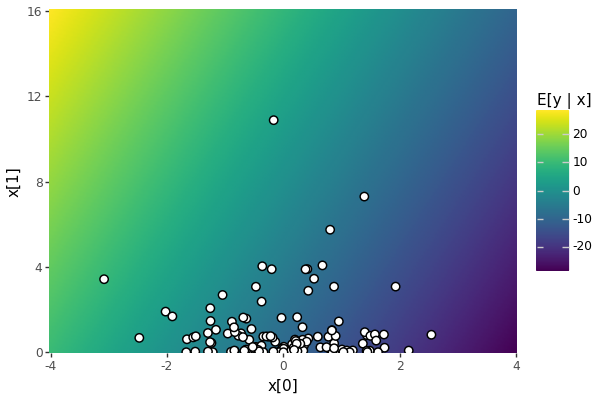
E[y | x] = alpha + x @ beta over 4 marginal standard deviations in x, where x[0] ~ normal(0, 1) and x[1] ~ chi_sq(1). The observed covariates overlaid as white disks.
4 Sampling with Stan
Now that we have defined a Stan program and simulated data, we can perform inference from the simulated data (pretending that we did not already know the parameters). We will use Stan’s defaults.
4.1 The CmdStanPy interface
We will use the Python interface CmdStanPy (Stan Development Team 2024), which makes an external system call to the reference command-line interface, CmdStan. Before that, we import the cmdstanpy package and make sure we have a compiled CmdStan installation and turn the logging level down to ERROR so that our output isn’t cluttered with progress messages.
import cmdstanpy as csp
from cmdstan_env import configure_cmdstan, cmdstan_model

configure_cmdstan()
CmdStan install directory: /home/runner/.cmdstan
Installing CmdStan version: 2.39.0
Downloading CmdStan version 2.39.0
Download successful, file: /tmp/tmptpftr59k
Extracting distribution
Unpacked download as cmdstan-2.39.0
Building version cmdstan-2.39.0, may take several minutes, depending on your system.
Installed cmdstan-2.39.0
Test model compilationHide/Show the code
import logging
csp.utils.get_logger().setLevel(logging.ERROR)
4.2 Transpilation and compilation
Once CmdStan is installed, transpiling the model to C++ and compiling the C++ is a one-liner.
m = cmdstan_model("linear-regression.stan")4.3 Sampling
Given the model m, sampling with Stan’s default parameters is a one liner. We call the sampler with the data variable simulated above, and we turn off progress bars to render in a paper.
fit = m.sample(data=data, show_progress=False)The variable data was defined above in the simulation. The call to sample() uses CmdStanPy’s default configuration parameters. By default, Stan uses the multinomial, biased-progressive no-U-turn sampler (Betancourt 2017), which invokes three stages of warmup (finding the bulk of the probability mass, estimating the inverse mass matrix, and estimating the step size). By default, Stan runs 1000 warmup and 1000 sampling iterations in 4 independent chains—this is often more than are necessary for model development and many applications.
4.4 Posterior summaries with CmdStanPy and ArviZ
Now that we have the fit, we can print a summary of the posterior from CmdStan, reducing its default number of digits printed.
summary_csp = fit.summary(sig_figs=3)
print(summary_csp)
Mean MCSE StdDev MAD 5% 50% 95% ESS_bulk \
lp__ 10.700 0.030000 1.3900 1.2300 8.120 11.00 12.400 2170.0
alpha -9.170 0.001040 0.0582 0.0579 -9.270 -9.17 -9.080 3180.0
beta[1] -4.810 0.000760 0.0467 0.0457 -4.890 -4.81 -4.730 3830.0
beta[2] 1.150 0.000568 0.0319 0.0326 1.090 1.15 1.200 3190.0
sigma 0.541 0.000556 0.0346 0.0351 0.487 0.54 0.601 3900.0
y_new[1] -10.600 0.008620 0.5580 0.5530 -11.500 -10.60 -9.650 4220.0
y_new[2] -16.300 0.008890 0.5600 0.5610 -17.200 -16.30 -15.400 3970.0
y_new[3] -17.800 0.008780 0.5460 0.5460 -18.700 -17.80 -16.900 3880.0
y_new[4] -8.530 0.009360 0.5420 0.5470 -9.400 -8.53 -7.620 3450.0
ESS_tail ESS_bulk/s R_hat
lp__ 2900.0 13600.0 1.0
alpha 2970.0 19900.0 1.0
beta[1] 2970.0 24000.0 1.0
beta[2] 2850.0 19900.0 1.0
sigma 2950.0 24400.0 1.0
y_new[1] 3740.0 26400.0 1.0
y_new[2] 3930.0 24800.0 1.0
y_new[3] 4060.0 24200.0 1.0
y_new[4] 4040.0 21600.0 1.0 The summary_csp variable provides programmatic access to the data this printed by default along with much more debugging and configuration information. The variable lp__ reported in the first row is the unnormalized log posterior density, the variables alpha, beta, and sigma report model parameters, and y_new reports the models posterior predictions. The remaining columns are defined per variable and include the posterior mean, Monte Carlo standard error, posterior standard deviation, mean absolute deviation (like standard deviation for medians), three quantiles (5%, 50%, and 95%), as well as some convergence diagnostics. The rank-normalized \widehat{R} statistic is reported in the last column, and the effective sample size in the bulk and tail of the density, as well as bulk effective sample size per second (where we see this all ran quickly); definitions of all of these are provided by Vehtari et al. (2021).
The summary shows that the model fits very well. While it doesn’t report timing, the effective sample size per second statistic lets you infer that this all ran in less than 0.1s. The \widehat{R} statistics are all below 1.005 and the effective sample sizes are all above 2000 with 4000 total sampling draws across four chains.
A very similar summary is available from the Python package ArviZ, which shares many developers with Stan. Using the method draws_xr(), CmdStanPy produces an Xarray (defined in package xarray) that can be directly consumed by ArviZ’s summary() function.
import arviz as az

fit_xr = fit.draws_xr()
summary_az = az.summary(fit_xr)
print(summary_az)
/home/runner/micromamba/envs/micromamba/lib/python3.11/site-packages/arviz/__init__.py:50: FutureWarning:
ArviZ is undergoing a major refactor to improve flexibility and extensibility while maintaining a user-friendly interface.
Some upcoming changes may be backward incompatible.
For details and migration guidance, visit: https://python.arviz.org/en/latest/user_guide/migration_guide.html mean sd hdi_3% hdi_97% mcse_mean mcse_sd ess_bulk \
alpha -9.174 0.058 -9.293 -9.075 0.001 0.001 3183.0
beta[0] -4.809 0.047 -4.894 -4.717 0.001 0.001 3833.0
beta[1] 1.148 0.032 1.088 1.207 0.001 0.000 3187.0
sigma 0.541 0.035 0.482 0.611 0.001 0.001 3897.0
y_new[0] -10.563 0.558 -11.649 -9.566 0.009 0.007 4225.0
y_new[1] -16.289 0.560 -17.348 -15.251 0.009 0.006 3969.0
y_new[2] -17.803 0.546 -18.762 -16.746 0.009 0.006 3877.0
y_new[3] -8.530 0.542 -9.535 -7.522 0.009 0.006 3453.0
ess_tail r_hat
alpha 2970.0 1.0
beta[0] 2969.0 1.0
beta[1] 2845.0 1.0
sigma 2953.0 1.0
y_new[0] 3744.0 1.0
y_new[1] 3930.0 1.0
y_new[2] 4056.0 1.0
y_new[3] 4043.0 1.0 The main difference is that ArviZ defaults to reporting 94% highest density intervals rather than traditional central intervals based on quantiles. ArviZ can be configured to include Stan’s quantile output, if desired and the highest-density interval changed to 90% coverage to match Stan’s output using NumPy’s quantile functions. These packages typically report 90% rather than 95% intervals because the standard error of quantile estimates increases dramatically in the tails (Bahadur 1966; Van der Vaart 1998).
summary_az_stan = az.summary(
    fit_xr,
    hdi_prob=0.9,
    stat_funcs={
        "q5": lambda x: np.quantile(x, 0.05),
        "q50": lambda x: np.quantile(x, 0.50),
        "q95": lambda x: np.quantile(x, 0.95),
    },
    extend=True
)
print(summary_az_stan)
mean sd hdi_5% hdi_95% mcse_mean mcse_sd ess_bulk \
alpha -9.174 0.058 -9.269 -9.080 0.001 0.001 3183.0
beta[0] -4.809 0.047 -4.884 -4.731 0.001 0.001 3833.0
beta[1] 1.148 0.032 1.098 1.202 0.001 0.000 3187.0
sigma 0.541 0.035 0.486 0.600 0.001 0.001 3897.0
y_new[0] -10.563 0.558 -11.410 -9.602 0.009 0.007 4225.0
y_new[1] -16.289 0.560 -17.176 -15.350 0.009 0.006 3969.0
y_new[2] -17.803 0.546 -18.712 -16.945 0.009 0.006 3877.0
y_new[3] -8.530 0.542 -9.363 -7.601 0.009 0.006 3453.0
ess_tail r_hat q5 q50 q95
alpha 2970.0 1.0 -9.274 -9.171 -9.083
beta[0] 2969.0 1.0 -4.885 -4.809 -4.732
beta[1] 2845.0 1.0 1.095 1.148 1.199
sigma 2953.0 1.0 0.487 0.540 0.601
y_new[0] 3744.0 1.0 -11.462 -10.572 -9.650
y_new[1] 3930.0 1.0 -17.208 -16.287 -15.374
y_new[2] 4056.0 1.0 -18.669 -17.819 -16.881
y_new[3] 4043.0 1.0 -9.398 -8.526 -7.620 5 Stan to C++ transpilation
A Stan program translates almost line-for-line to a C++ class that implements all the interfaces around a model required for log density evaluation, posterior predictive quantity generation, and variable transforms (Stan Development Team 2025).
5.1 Stan’s block structure
Functions block: Each function in the functions block is translated to a C++ function that is templated flexibly enough to allow automatic differentiation. The main limitation to Stan’s functions is that they cannot cross blocks and they cannot introduce block-level variables such as data or parameters; a secondary limitation is that arguments must be real or integer based. Thus it is not possible to define functions like the built-in ODE solvers that take functions as arguments.
Data and transformed data blocks: Each data declaration in the data block is translated to an instance variable of the generated class. The data block can only contain declarations, and thus behaves like the signature for the data ingestion function. The transformed data block is executed after the data is read in as the model object is being constructed. After the model object is constructed with the data, it remains immutable to allow safe multi-threaded application.
Parameter and transformed parameter blocks: The log density function is defined for unconstrained inputs gathered into a vector. The first part of the function unpacks the entries of that vector, applies the constraining transform to define constrained variables locally, then adds the log Jacobian determinant to the Jacobian accumulator to adjust for the change-of-variables making up the constraint. Transformed parameters also define local variables. Everything executes serially as coded in the Stan program.
Model block: The rest of the body of the log density function is the line-by-line translation of Stan’s model block. Each distribution and target increment statement increments the log density accumulator, which is returned as the value of the function. Everything is templated generally enough and coded in the underlying math library to allow automatic differentiation; the automatic differentiation code dominates the project in terms of size and presents the most challenges to developer recruitment because of its modern C++ architecture (Carpenter et al. 2015).
Generated quantities block: This block is motivated by the goal of providing efficient forward-simulated predictive inferences. The generated quantities block translates to a function that maps the parameters and a random number generator to the variables of interest. These are gathered by this function along with the parameters and transformed parameters to form vector output. The names of all the parameters define the columns of output and output is on the constrained scale where the user and Stan program model block operate.
5.2 Stan’s transpiled C++ model class
Stan programs are transpiled to C++, and then the C++ is compiled down to machine instructions. The C++ class generated for the model has the following signatures, which have been simplified to remove debugging traces, template traits restrictions, and some fine-grained control parameters. This is the same interface that is exposed by BridgeStan in Python, R, Julia, C, and Rust (Roualdes et al. 2023).
namespace lr_model_namespace {

class lr_model : model_base<lr_model> {
  // data, transformed data
  int N, N_new, P;    MatrixXd x;
  VectorXd y;         MatrixXd x_new;

  // read data from c, compute transformed data
  linear_regression_model(var_context& c, int seed,
                          ostream* msgs);

  // log density type T, propto drops constants, jacobian adjusts
  template <bool propto, bool jacobian, typename T>
  Vector<T> log_prob(Vector<T>& params, ostream* msgs) const;

  // evaluate generated quantities and write csv
  template <typnename RNG>
  void write(RNG& rng, const VectorXd& params,
             ostream* csv_stream) const;


  string model_name() const noexcept;

  void unconstrain(const VectorXd& constrained_params,
                   VectorXd& unconstrained_params) const;
  void constrain(var_context& vars, VectorXd& constrained_params,
                 ostream* msgs) const;

  void param_names(vector<string>& names) const;
  void constrained_param_names(vector<string>& names) const;
};
} // lr_model_namespace

// global namespace factory for lr_model
model_base& new_model(var_context& c, int seed, ostream* msgs);
The data variables are specified in the data block in the Stan program. Here, we have the sizes, the covariate matrices (x plus x_new for posterior prediction), and the outcomes (y). The constructed C++ class is immutable and provides several methods, the most central of which is an unconstrained (in the sense of having support over all of \mathbb{R}^D) log density function that is templated in order to support automatic differentiation (Carpenter et al. 2015). In math, the constraining transform maps (\alpha, \beta, \sigma^\text{u}) to (\alpha, \beta, \exp(\sigma^\text{u})). The transforms are independent and the first two are the identity, so the Jacobian determinant works out to \exp(\sigma^\text{u}). Thus the additive change-of-variables adjustment on the log scale is just \log \exp(\sigma^\text{u}) = \sigma^\text{u}.
The model block defines a density function p over constrained parameters. Although Stan can be used to sample from any density, it is typically used to code the unnormalized posterior log density of a Bayesian mode. Densities are read elementwise, with scalar arguments being broadcast where necessary. With this translation, the unnormalized log posterior over the constrained variables defined by the Stan program’s model block is \log p(\alpha, \beta, \sigma \mid x, y) = \log \textrm{normal}(\alpha \mid 0, 5) + \sum_{p=1}^P \textrm{normal}(\beta_p \mid 0, 2.5) \\ + \log \textrm{exponential}(\sigma \mid 0.5) + \sum_{n=1}^N \textrm{normal}(y_n \mid \alpha + \beta \cdot x_n, \sigma). The corresponding unconstrained log density over which inference is performed, adds the log Jacobian adjustment for the change of variables, \log p^\text{u}(\alpha, \beta, \sigma^\text{u} \mid x, y) = \log p(\alpha, \beta, \exp(\sigma^\text{u}) \mid x, y) + \sigma^\text{u}.
The transpiled C++ code implementing the log density function performs the following sequence of operations, which directly follows the Stan program. The typing, logging, debugging traces, message I/O, and name mangling have all been simplified.
template <bool propto, bool jacobian, typename T>
inline auto log_prob(Vector<T>& params) const {
  Accumulator<T> accum;

  // transpiled parameters block
  T log_jacobian;
  Deserializer<T> in(params)
  auto alpha = in.template read<T>();
  auto beta = in.template read<Vector<T>>(P);
  auto sigma = in__.template read_constrain_lb<T, jacobian>(0, log_jacobian);
  accum.add(log_jacobian);

  // transpiled model block
  accum.add(normal_lpdf<propto>(alpha, 0, 5));
  accum.add(normal_lpdf<propto>(beta, 0, 2.5));
  accum.add(exponential_lpdf<propto>(sigma, 0.5));
  accum.add(normal_lpdf<propto>(y, add(alpha, multiply(beta, x))), sigma);

  return accum.sum();
}
The read methods of the deserializer read the next variable from the sequence of parameters, perform any necessary constraining transform and add any Jacobian adjustment to lp, controlled by the flag jacobian. Arithmetic in the Stan program is replaced with overloaded internal library calls add and multiply which can handle vectors and scalars. There is implicit broadcasting and internal summation in the normal_lpdf log density function. When applied to a vector like beta or y, it sums the log densities of the components, broadcasting any scalar arguments as necessary. The accumulator collects terms and then its method sum returns a flattened autodiff tree with a single root pointing to all the terms with implicit unit derivatives.
To support the changes of variables for reporting constrained output, the compiled C++ code exposes the constraining transform and its Jacobians. For initialization from constrained parameters, there is a matching unconstraining transform. The model class also supplies methods for determining the shape and names of the constrained and unconstrained parameters.
The final component of a compiled Stan model is a function to perform predictive inference as defined by the generated quantities block (this can also be done post-hoc with a new program and generated quantities block). In particular, the model compiles a generated quantities function write() that takes a random number generator and produces the output defined in the generated quantities block purely by forward sampling without the need for any automatic differentiation.
6 Coding models directly in JAX
In this section, we will translate the functionality provided by Stan’s C++ class directly into a more functional JAX style. It’s much simpler than Stan’s transpiled C++ code because of the built-in serialization and optimization of PyTree and the binding of data. In the next section, we will wrap up some utility functions to make it much easier to achieve the same functionality.
6.1 Linear regression directly in JAX
This section provides one way to code our linear regression model directly in JAX. We will start by importing the libraries we need, which include JAX’s version of NumPy, JAX’s random number generator, and the stats library from JAX’s version of SciPy. Finally, we import the Blackjax library for sampling. We first import all of JAX itself as we will need it for just-in-time compilation.
import jax
import jax.numpy as jnp
import jax.random as jrd
from jax.scipy import stats
import blackjax

from examples.util import positive, real
Before we begin, we will also convert the Python and NumPy data types to JAX.
x = jnp.array(data["x"])
y = jnp.array(data["y"])
x_new = jnp.array(data["x_new"])
6.2 The model parameters
Stan’s log density function operates over the vector of parameters declared in the Stan program’s parameters block. To take advantage of JAX’s built-in serialization and optimization of PyTree, we construct a dictionary over all parameters which defines their shapes and dtypes.
params = {
    "alpha": real(),
    "beta": real(shape=x.shape[1]),
    "sigma": positive(),
}
6.3 The untransformed log posterior in JAX
The log density function from the Stan model block can then be translated almost line by line into JAX; we only break out the definition of mu for readability—it could have been a nested expression.
def log_posterior(params):
    lp = 0.0
    lp += jnp.sum(stats.norm.logpdf(params["alpha"], loc=0.0, scale=5.0))
    lp += jnp.sum(stats.norm.logpdf(params["beta"], loc=0.0, scale=2.5))
    lp += jnp.sum(stats.expon.logpdf(params["sigma"], scale=1.25))
    mu = params['alpha'] + x @ params["beta"]
    lp += jnp.sum(stats.norm.logpdf(y, loc=mu, scale=params["sigma"]))
    return lp
The log_posterior function binds the covariate matrix x and the outcome vector y from the top-level environment. An alternative would have been to bind a JAX conversion of top-level container data, but we never need the encapsulated data, so just define the variables directly. The log probability density functions are implemented in JAX’s version of SciPy’s stats library. Unlike in Stan, where density functions automatically reduce by summation, the functions in stats.norm return JAX arrays, which are here summed by JAX’s version of NumPy before being added to the target log density accumulator lp.
The parameters themselves are read out of the argument dictionary. While this may appear inefficient, JAX’s just-in-time (JIT) compiler is smart enough to reduce the dictionary lookups to direct accesses at run time.
6.4 Transforms and their inverses in JAX
Before we can use this log posterior for sampling, we need a few support functions. To mirror Stan, the sampler needs to work on the transformed scale. Here, as in most programs, the transform maps constrained variables to unconstrained ones. In our regression example, the scale, which is constrained to (0, \infty), is log-transformed so that the transformed scale ranges over the whole real number line, (-\infty, \infty).
We will start with the transform, which is only needed in practice for initializations from untransformed parameter values. In the linear regression example, the transform maps the regression coefficients to themselves and the scale to the log scale.
def transform(params):
    t_alpha = params["alpha"]
    t_beta = jnp.array(params["beta"])
    t_sigma = jnp.log(params["sigma"])
    t_params = { "alpha": t_alpha, "beta": t_beta, "sigma": t_sigma }
    return t_params
The transform() function could have been implemented in one line. Instead, we chose to follow a variable-by-variable pattern that will make it easier to automate later.
The inverse transform is needed at runtime to map the transformed variables back to their untransformed state so that the log posterior may be applied. For the inverse transform, any adjustment to ensure the implied distribution on the untransformed parameter space is uniform is returned along with the transformed parameters. Typically, this is a Jacobian determinant to adjust for a bijective change-of-variables. We use the same variable names for both transformed and untransformed parameters. The adjustment for the log change of variables here is just the log scale itself, as we derived above. To keep the code structure regular and to ease the transition to automation, we use a log adjustment variable that is initialized to zero and updated after each inverse transform.
def inv_transform(t_params):
    log_adjust = 0.0
    alpha = t_params["alpha"]
    beta = jnp.array(t_params["beta"])
    sigma = jnp.exp(t_params["sigma"])
    log_adjust += t_params["sigma"]
    params = { "alpha": alpha, "beta": beta, "sigma": sigma }
    return params, log_adjust
6.5 The tranformed log density in JAX
The transformed log posterior function we will use for sampling can be defined to apply the inverse transform and add the adjustment.
def log_posterior_transformed(t_params):
    params, log_adjust = inv_transform(t_params)
    log_post = log_posterior(params)
    return log_adjust + log_post
6.6 Random initialization in JAX
Following Stan, we need a way to generate a transformed random initialization. Here we use JAX’s version of SciPy’s stats.random library (imported above as jrd).
def random_init_transformed(key):
    key0, key1, key2 = jrd.split(key, 3)
    t_alpha = jrd.normal(key0)
    t_beta = jrd.normal(key1, shape=(2,))
    t_sigma = jrd.normal(key2)
    t_params = { "alpha": t_alpha, "beta": t_beta, "sigma": t_sigma }
    return t_params
The random number generators are supplied with shapes for variables that are not scalars. Let’s generate an initialization.
seed = 441_582
key = jrd.key(seed)
init_key, nuts_key = jrd.split(key, 2)
t_params_init = random_init_transformed(init_key)
print(f"{t_params_init=}")
t_params_init={'alpha': Array(-0.48995897, dtype=float32), 'beta': Array([0.19053426, 1.4290651 ], dtype=float32), 'sigma': Array(0.23013926, dtype=float32)}As a consistency check, we verify that the parameters we used to generate data are round-trippable through the transform and inverse transform.
params_init, log_adjust = inv_transform(t_params_init)
t_params_init_round_trip = transform(params_init)

print(f"{params_init=}")
print(f"{log_adjust=}")
print(f"{t_params_init_round_trip=}")
params_init={'alpha': Array(-0.48995897, dtype=float32), 'beta': Array([0.19053426, 1.4290651 ], dtype=float32), 'sigma': Array(1.2587752, dtype=float32)}
log_adjust=Array(0.23013926, dtype=float32)
t_params_init_round_trip={'alpha': Array(-0.48995897, dtype=float32), 'beta': Array([0.19053426, 1.4290651 ], dtype=float32), 'sigma': Array(0.23013921, dtype=float32)}The round trip arithmetic is not exact for sigma, because JAX works with 32-bit float types (float32) by default,
6.7 Sampling in Blackjax
Before sampling, we will define a top-level Markov chain sampler and then we will instantiate it with the NUTS transition kernel configured to run in a way that matches Stan’s defaults.
def random_markov_chain(key, kernel, init_state, num_draws):
    @jax.jit
    def one_step(state, key):
        state, _ = kernel(key, state)
        return state, state
    keys = jrd.split(key, num_draws)
    _, states = jax.lax.scan(one_step, init_state, keys)
    return states

def nuts_sample(key, log_density, init_position, num_draws):
    init_key, warmup_key, sample_key = jrd.split(key, 3)
    warmup = blackjax.window_adaptation(blackjax.nuts, log_density)
    (state, params), _ = warmup.run(warmup_key, init_position, num_steps=num_draws)
    kernel = blackjax.nuts(log_density, **params).step
    states = random_markov_chain(sample_key, kernel, state, num_draws)
    draws = states.position
    return draws
Working outward, the nested function one_step takes one step of a Markov chain from a given state and returns the next state. It uses a supplied transition kernel and random key. It starts from the specified initial state and produces the specified number of draws. It uses JAX’s lax scan to execute the loop, repeatedly applying the one-step transition function. The NUTS sample function is the top level caller. it takes a PRNG key, the target log density, an initial position, and a number of draws that specifies the number of warmup draws and the number of sampling draws. It uses Blackjax’s windowed warmup, as defined by Stan, then the NUTS sampler. The algorithm was defined to mirror Stan’s reference implementation.
We’ve already generated a transformed initialization t_params_init, so all that remains is to call the sample function.
num_draws = 1_000

t_draws = nuts_sample(nuts_key, log_posterior_transformed, t_params_init, num_draws)
6.8 Posterior analysis in JAX
We will do just a bit of posterior analysis manually to make sure we’re on the right track. Before that, we need to inverse transform our draws. We’ll do that with a vectorized function and a single call.
def inv_transform_draws(t_draws):
    draws = {
        "alpha": t_draws["alpha"],
        "beta": t_draws["beta"],
        "sigma": jnp.exp(t_draws["sigma"]),
    }
    return draws

draws = inv_transform_draws(t_draws)
Now we can perform the posterior analysis and see that it matches the results from Stan to within the tolerances to be expected from the standard errors.
import functools

posterior_means = jax.tree.map(functools.partial(jnp.mean, axis=0), draws)
posterior_stds = jax.tree.map(functools.partial(jnp.std, axis=0), draws)
print(f"{posterior_means=}")
print(f"{posterior_stds=}")
posterior_means={'alpha': Array(-9.174101, dtype=float32), 'beta': Array([-4.808164 , 1.1481543], dtype=float32), 'sigma': Array(0.53950995, dtype=float32)}
posterior_stds={'alpha': Array(0.05411908, dtype=float32), 'beta': Array([0.04893167, 0.03037017], dtype=float32), 'sigma': Array(0.03622, dtype=float32)}6.9 Posterior predictive quantities in JAX
In Stan, posterior predictive quantities are typically defined in the generated quantities block. In JAX, we can lazily define posterior predictive functions after sampling and efficiently map them over the posterior draws. Here’s a function that matches the generated quantities block defined in the Stan implementation of linear regression. We have already converted the covariates x_new to JAX above.
data_new = { "x_new": x_new }

def posterior_predictive(key, params):
    mu = params["alpha"] + data_new["x_new"] @ params["beta"]
    z = jax.random.normal(key, shape=mu.shape)
    y_new = mu + params["sigma"] * z
    return {"y_new": y_new}
Unlike the write() function in Stan’s transpiled C++ class, there is no need to inverse transform—we already have the parameters on the natural scale at this point and can just pass them to the predictive function.
def posterior_predictive_draws(key, draws):
    N = draws["alpha"].shape[0]
    keys = jax.random.split(key, N)
    return jax.vmap(posterior_predictive, in_axes=(0, 0))(keys, draws)

key, gq_key = jrd.split(key, 2)
pred_draws = posterior_predictive_draws(gq_key, draws)
The vmap is the way that JAX maps a function in parallel. The call above is equivalent to
results = []
for i in range(S):
    results.append(posterior_predictive(keys[i], params_draws[i]))
return results
The specification in_axes=(0, 0) tells the application of posterior_predictive to bind to the first argument (i.e., to index position 0).
We can summarize the results as before and verify they line up with the output from Stan’s generated quantities block.
posterior_pred_means = jax.tree.map(functools.partial(jnp.mean, axis=0), pred_draws)
posterior_pred_stds = jax.tree.map(functools.partial(jnp.std, axis=0), pred_draws)
print(f"{posterior_pred_means=}")
print(f"{posterior_pred_stds=}")
posterior_pred_means={'y_new': Array([-10.565608, -16.299402, -17.768396, -8.535892], dtype=float32)}
posterior_pred_stds={'y_new': Array([0.5454136 , 0.5331531 , 0.5449212 , 0.55034816], dtype=float32)}6.10 Key differences between the Stan and JAX implementations
Some of the bigger differences between Stan and its JAX implementation are as follows.
- There are no data declarations. The functions simply bind (i.e., close over) the data variables
xandy(i.e., it reads them from the environment where it was defined); we will shortly show how to abstract this into a function. - JAX does not require parameters to be serialized. With the wizardry of PyTree, Blackjax and other JAX-based packages can work directly with the
log_probfunction without any need for serialization. If serialized log density functions are needed elsewhere, they are convertible with a single function call as we show below. - There is no need to work with accumulators—JAX’s just-in-time compilation is sufficient to optimize sequences of operations at the XLA substrate to which JAX is compiled.
- The generated quantities are not part of the basic model specification, but rather flexibly called later. While we could have done the same with Stan, the Stan functions are not available in either R or Python, making this another two-language problem. Furthermore, JAX’s ability to efficiently scan accelerates posterior predictive inference in JAX.
- There are no function blocks because plain old Python functions can be applied to JAX objects. The only caveat is that these functions will be traced, so cannot contain any runtime branching on parameter values.
Aside from the verbosity of all the namespace qualifiers and the need for all the intermediate calls to sum, the biggest obstacle to writing code this way is having to manually deal with the transforms and inverse transforms. Our goal is to make it as simple as Stan in the next section.
7 Linear regression in JAX with densejax
The Stan linear regression can be translated almost line for line into Python using densejax.
from densejax import (
    real, positive, normal, exponential, normal_rng, model
)

def linear_regression(x, y, x_new):
    N, P = x.shape

    parameters = {
      'a': real(),
      'b': real(size=P),
      's': positive()
    }

    def log_density(a, b, s):
        lp = 0
        lp += normal(a, 0, 2)
        lp += normal(b, 0, 1)
        lp += exponential(s, 0.5)
        lp += normal(y, a + x @ b, s)
        return lp

    def generate(rng, a, b, s):
        y_new = normal_rng(rng, a + x_new @ b, s)
        return { 'y_new': y_new }

    return model(parameters, log_density, generate)
After calling this function with data, the resulting model object is feature equivalent to all the manual code written above for transforming parameters and performing initialization. It mirrors the C++ object produced by Stan (also the model object produced by BridgeStan (Roualdes et al. 2023)). Because these simple functions generate fully JAX-embedded code, the log density function can be automatically differentiated and all of the functions can be just-in-time compiled.
7.1 Abstracting parameter transformations
In order to automate the transformation functionality that were coded manually above, we introduce the idea of a “parameter specification” (the parameters dictionary in the code) which provides all the information about how the parameters should be transformed. The leaves of this parameter specification are simple classes like positive, which is reproduced here in full:
class positive(ParameterConstraint):
    def __init__(self, shape=(), dtype=jnp.float32):
        self.shape = shape
        self.dtype = dtype

    def inverse_transform(self, x):
        return jnp.exp(x)

    def transform(self, y):
        return jnp.log(y)

    def jacobian(self, x):
        return jnp.sum(x)
The densejax package provides a menu of existing transforms, but the above class is designed to be simple enough to be easily extensible.
The real class is simply a transform that has the identity for both sides of the transformation; we rely on JAX’s jit compiler to remove any overhead from this implementation style.
Turning this parameter spec into functions that perform the inverse transforms, transforms, and (possibly random) initialization is trivial. All of these reduce to simple map-like operations over the specification and the provided parameter values where required.
The majority of the code in densejax consists of these transformation classes, utility functions consuming them, and the small wrappers provided for common distributions like normal as seen above.
7.2 Simplifying inference
The model object remains general enough for use in any gradient based sampler implemented in JAX; the one-liner
log_posterior_transformed = jax.jit(model.log_density)would be enough to use blackjax in the same manner as above.
However, bundling more of the desired functionality into one object allows for more turn-key helpers. Consider the following new definition of nuts_sample:
def nuts_sample(key, model, num_draws, init=None):
    log_density = jax.jit(model.log_density)

    init_key, warmup_key, sample_key = jrd.split(key, 3)

    if init is None:
        init_position = model.initialize_random(init_key)
    else:
        init_position = model.initialize(init)

    warmup = blackjax.window_adaptation(blackjax.nuts, log_density)
    (state, params), _ = warmup.run(warmup_key, init_position, num_steps=num_draws)

    kernel = blackjax.nuts(log_density, **params).step
    constrain = jax.jit(model.inv_transform)
    @jax.jit
    def one_step(state, key):
        state, _ = kernel(key, state)
        return state, constrain(**state.position)

    keys = jrd.split(sample_key, num_draws)
    _, draws = jax.lax.scan(one_step, state, keys)

    return draws
This version of nuts_sample has the advantage over the previous that both the input initial values and the returned draws are in the model space. The user on the outside does not need to worry about transforming the initial values and inverse-transforming the results.
We could have written nuts_sample to do this for us before, if we had been willing to pass it additional arguments; the model class makes it very natural to define the most useful version out of the box.
Given these snippets, one can recreate the complete sampling workflow from the prior section with the following brief code:
seed = 441_582
key = jrd.key(seed)

model = linear_regression(x, y, x_new)
num_draws = 1_000
draws = nuts_sample(key, model, num_draws)

mean = functools.partial(jax.tree.map(functools.partial(jnp.mean, axis=0)))
std = functools.partial(jax.tree.map(functools.partial(jnp.mean, axis=0)))

print(f"{mean(draws)=}")
print(f"{std(draws)=}")

# posterior predictive
key, gq_keys = jrd.split(key, 1+num_draws)
pred_draws = jax.vmap(model.forward, in_axes=(0, 0))(keys,draws)

print(f"{mean(pred_draws)=}")
print(f"{std(draws)=}")
References
Bahadur, R Raj. 1966. “A Note on Quantiles in Large Samples.” The Annals of Mathematical Statistics 37 (3): 577–80.
Betancourt, Michael. 2017. “A Conceptual Introduction to Hamiltonian Monte Carlo.” arXiv 1701.02434.
Blondel, Mathieu, Quentin Berthet, Marco Cuturi, et al. 2021. “Efficient and Modular Implicit Differentiation.” arXiv 2105.15183.
Cabezas, Alberto, Adrien Corenflos, Junpeng Lao, et al. 2024. “BlackJAX: Composable Bayesian Inference in JAX.” arXiv 2402.10797.
Carpenter, Bob, Andrew Gelman, Matthew D Hoffman, et al. 2017. “Stan: A Probabilistic Programming Language.” Journal of Statistical Software 76: 1–32.
Carpenter, Bob, Matthew D Hoffman, Marcus Brubaker, Daniel Lee, Peter Li, and Michael Betancourt. 2015. “The Stan Math Library: Reverse-Mode Automatic Differentiation in C++.” arXiv 1509.07164.
Cook, Samantha, Andrew Gelman, and Donald B. Rubin. 2006. “Validation of Software for Bayesian Models Using Posterior Quantiles.” Journal of Computational and Graphical Statistics 15 (3): 675–92.
DeepMind, Igor Babuschkin, Kate Baumli, et al. 2020. The DeepMind JAX Ecosystem. Released. http://github.com/deepmind.
Dillon, Joshua V, Ian Langmore, Dustin Tran, et al. 2017. “Tensorflow Distributions.” arXiv 1711.10604.
Dinh, Laurent, Jascha Sohl-Dickstein, and Samy Bengio. 2016. “Density Estimation Using Real NVP.” arXiv 1605.08803.
Doucet, Arnaud, Nando De Freitas, and Neil Gordon. 2001. “An Introduction to Sequential Monte Carlo Methods.” In Sequential Monte Carlo Methods in Practice. Springer.
Gabry, Jonah, Daniel Simpson, Aki Vehtari, Michael Betancourt, and Andrew Gelman. 2019. “Visualization in Bayesian Workflow.” Journal of the Royal Statistical Society Series A: Statistics in Society 182 (2): 389–402.
Ge, Hong, Kai Xu, and Zoubin Ghahramani. 2018. “Turing: A Language for Flexible Probabilistic Inference.” International Conference on Artificial Intelligence and Statistics, 1682–90.
Gelman, Andrew, John B Carlin, Hal S Stern, David B Dunson, Aki Vehtari, and Donald B Rubin. 2013. Bayesian Data Analysis. Third. Chapman; Hall/CRC.
Gelman, Andrew, Aki Vehtari, Daniel Simpson, et al. 2020. “Bayesian Workflow.” arXiv 2011.01808.
Gorinova, Maria I, Andrew D Gordon, and Charles Sutton. 2019. “Probabilistic Programming with Densities in SlicStan: Efficient, Flexible, and Deterministic.” Proceedings of the ACM on Programming Languages 3 (POPL): 1–30.
Guennebaud, Gaël, and Benoît Jacob. 2010. “Eigen: A C++ linear algebra library.” Eurographics/CGLibs.
Hastings, W. K. 1970. “Monte Carlo Sampling Methods Using Markov Chains and Their Applications.” Biometrika 57: 97–109.
Heek, Jonathan, Anselm Levskaya, Avital Oliver, et al. 2024. Flax: A Neural Network Library and Ecosystem for JAX. V. 0.12.3. Released. http://github.com/google/flax.
Hoffman, Matthew D, and Andrew Gelman. 2014. “The No-U-Turn Sampler: Adaptively Setting Path Lengths in Hamiltonian Monte Carlo.” Journal of Machine Learning Research 15 (1): 1593–623.
Horowitz, Alan M. 1991. “A Generalized Guided Monte Carlo Algorithm.” Physics Letters B 268 (2): 247–52.
Josuttis, Nicolai M. 2012. The C++ Standard Library: A Tutorial and Reference. Addison-Wesley.
Kidger, Patrick. 2021. “On Neural Differential Equations.” PhD thesis, University of Oxford.
Kochkov, Dmitrii, Jamie A. Smith, Ayya Alieva, Qing Wang, Michael P. Brenner, and Stephan Hoyer. 2021. “Machine Learningaccelerated Computational Fluid Dynamics.” Proceedings of the National Academy of Sciences 118 (21). https://doi.org/10.1073/pnas.2101784118.
Kucukelbir, Alp, Dustin Tran, Rajesh Ranganath, Andrew Gelman, and David M Blei. 2017. “Automatic Differentiation Variational Inference.” Journal of Machine Learning Research 18 (14): 1–45.
Kumar, Ravin, Colin Carroll, Ari Hartikainen, and Osvaldo Martin. 2019. “ArviZ a Unified Library for Exploratory Analysis of Bayesian Models in Python.” Journal of Open Source Software 4 (33): 1143.
Lunn, David, Chris Jackson, Nicky Best, Andrew Thomas, and David Spiegelhalter. 2012. The BUGS Book: A Practical Introduction to Bayesian Analysis. CRC Press.
Lunn, David, David Spiegelhalter, Andrew Thomas, and Nicky Best. 2009. “The BUGS Project: Evolution, Critique and Future Directions.” Statistics in Medicine 28 (25): 3049–67.
Margossian, Charles C. 2023. “General Adjoint-Differentiated Laplace Approximation.” arXiv 2306.14976.
Maskell, Simon. 2024. Running Multiple Short MCMC Chains on a GPU Using JAX for Fast Inference with Stan. YouTube! video. https://www.youtube.com/watch?v=KpLZEYX8MpY.
Murray, Iain, Ryan Adams, and David MacKay. 2010. “Elliptical Slice Sampling.” Proceedings of the 13th International Conference on Artificial Intelligence and Statistics, 541–48.
Paulin, Daniel. 2015. “Concentration Inequalities for Markov Chains by Marton Couplings and Spectral Methods.” Electronic Journal of Probability 20 (79): 1–32. https://doi.org/10.1214/EJP.v20-4039.
Phan, Du, Neeraj Pradhan, and Martin Jankowiak. 2019. “Composable Effects for Flexible and Accelerated Probabilistic Programming in NumPyro.” arXiv 1912.11554.
Plummer, Martyn. 2003. “JAGS: A Program for Analysis of Bayesian Graphical Models Using Gibbs Sampling.” Proceedings of the 3rd International Workshop on Distributed Statistical Computing (Vienna, Austria) 124: 1–10.
Roberts, Gareth O, and Jeffrey S Rosenthal. 2004. “General State Space Markov Chains and MCMC Algorithms.” Probability Surveys 1: 20–71.
Robnik, Jakob, Reuben Cohn-Gordon, and Uroš Seljak. 2025. “Metropolis Adjusted Microcanonical Hamiltonian Monte Carlo.” arXiv 2503.01707.
Roualdes, Edward A, Brian Ward, Bob Carpenter, Adrian Seyboldt, and Seth D Axen. 2023. “BridgeStan: Efficient in-Memory Access to the Methods of a Stan Model.” Journal of Open Source Software 8 (87): 5236.
Rubin, Donald B. 1996. “Multiple Imputation After 18+ Years.” Journal of the American Statistical Association 91 (434): 473–89.
Salvatier, John, Thomas V Wiecki, and Christopher Fonnesbeck. 2016. “Probabilistic Programming in Python Using PyMC3.” PeerJ Computer Science 2: e55.
Sountsov, Pavel, Colin Carroll, and Matthew D Hoffman. 2024. “Running Markov Chain Monte Carlo on Modern Hardware and Software.” arXiv 2411.04260.
Stan Development Team. 2024. CmdStanPy. V. 1.3.0. Released. https://doi.org/10.5281/zenodo.5733022.
Stan Development Team. 2025. Stan Reference Manual. Version 2.38. Stan Project. https://mc-stan.org/docs/reference-manual/.
Valpine, Perry de, Daniel Turek, Christopher J Paciorek, Clifford Anderson-Bergman, Duncan Temple Lang, and Rastislav Bodik. 2017. “Programming with Models: Writing Statistical Algorithms for General Model Structures with NIMBLE.” Journal of Computational and Graphical Statistics 26 (2): 403–13.
Van der Vaart, A W. 1998. Asymptotic Statistics. Cambridge Series on Statistical and Probabilistic Mathematics 3. Cambridge University Press.
Vehtari, Aki, Andrew Gelman, and Jonah Gabry. 2017. “Practical Bayesian Model Evaluation Using Leave-One-Out Cross-Validation and WAIC.” Statistics and Computing 27 (5): 1413–32.
Vehtari, Aki, Andrew Gelman, Daniel Simpson, Bob Carpenter, and Paul-Christian Bürkner. 2021. “Rank-Normalization, Folding, and Localization: An Improved R-Hat for Assessing Convergence of MCMC (with Discussion).” Bayesian Analysis 16 (2): 667–718.
Zhang, Lu, Bob Carpenter, Andrew Gelman, and Aki Vehtari. 2022. “Pathfinder: Parallel Quasi-Newton Variational Inference.” Journal of Machine Learning Research 23 (306): 1–49.
Reuse
CC-BY-4.0